Demystifying Attention!
In this article, I will introduce the most common form of attention (also known as soft-attention or additive attention), initially proposed by (Bahdanau et al.) to improve the performance of basic encoder-decoder architecture. I plan to write all different types of attention in a separate article, and therefore the goal of this article will not be to introduce various forms of attention and differentiate among them. Furthermore, in this article, I aim first to provide the motivation, followed by the relevant mathematical equations to help deepen the understanding of the topic.
- Basic Encoder-Decoder Architecture
- Limitations of Basic Encoder-Decoder Architecture
- Solution? Decoder with Attention
- References
Basic Encoder-Decoder Architecture
A sequence-to-sequence model was first proposed by (Sutskever et al. 2014) in the form of basic encoder-decoder architecture. They offered a first general end-to-end approach to sequence learning, i.e., mapping input sequence to target sequence. In a nutshell, an encoder takes a sequence in input and maps that into a context vector consumed by a decoder to generate a target sequence.
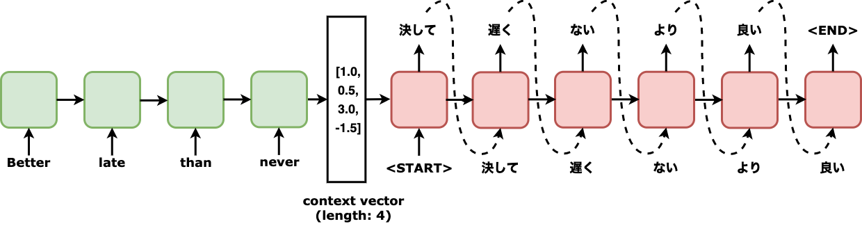
Fig. 1 Abstractive example of encoder-decoder architecture usage translating an English sentence “Better late than never” to Japanese “決して 遅く ない より 良い.”
To appreciate the magical power of attention, it is essential to understand the working of both the encoder and decoder. Once you know how these two components work, it will be easier to comprehend their limitations, leading us to the motivation for attention mechanism and how it eliminates those limitations. Let’s jump in to understand how encoder and decoder work!
Encoder
An encoder in basic encoder-decoder architecture reads the input sequence \(x\) = \(x_{1}, x_{2}, .. x_{Tx}\) and compresses that to a vector of fixed-length (dimension). This fixed-length vector is also known as context vector \(c\). The motivation for this transformation is to map the input sequence to a language-agnostic representation so that later decoder can generate the target sequence conditioned on this language-agnostic representation (i.e., context vector generated by the encoder). The next question that arises is how does the encoder perform this compression? The most common approach for such compression is to use a Recurrent Neural Network (RNN) to take input sequence one word at a time and generate an encoded representation in the form of hidden state \(h\) for each input word such that.
\[h_{i}=f\left(x_{i}, h_{i-1}\right) \label{eq:encoder_state}\]In \eqref{eq:encoder_state} \(i\) represents the time stamp, \(h_{i} \in \mathbb{R}^{n}\) is an n-dimensional hidden state of the encoder at the i-th timestamp. And \(f\) is a nonlinear function (e.g., LSTM). Theoretically, in \eqref{eq:encoder_state}, the encoder is computing an encoded representation of all the words seen in the input sequence. However, practically the representation is highly biased towards only recently seen words. When the encoder has completed reading all the words in the input sequence, we should have this hidden representation equal to the number of words in the input sequence.
We saw how the encoder calculates the encoded representation at each time step of the input sequence. Now the question arises, how shall one combine the individual encoded representations to form a context vector, i.e., a single piece of information which the decoder can use to start generating the target sequence? To put it mathematically in \eqref{eq:context_vector} we want a function \(q\) which can transform all the encoded representations i.e. \(h_{1}, h_{2}, .., h_{T_{x}}\) into a single context vector \(c\).
\[c=q\left(\left\{h_{1}, \cdots, h_{T_{x}}\right\}\right) \label{eq:context_vector}\]The obvious next question is, what is a good choice of this function \(q\) ? Well in (Sutskever, et al. 2014) they proposed a logically simple function for \(q\) described in \eqref{eq:encoder_context_vector}. In essence, they decided to encode variable-length input sequence into a fixed-length vector based on the last encoded representation i.e. \(h_{T_x}\).
\[c=q=h_{Tx} \label{eq:encoder_context_vector}\]This means the context vector was a copy of the last hidden state of the encoder. One might think, why did they decide to use only the last hidden state and not the hidden states in the previous steps? If you think the intuition behind this formulation is simple, the encoder, when consuming the previous word in the input sequence, should have compressed all the essential information from all the words seen so far (i.e., complete input sequence) down into a single hidden vector. This property of a vector to consist of all the essential information from the input is what we were looking for in a context vector. Therefore it made sense to propose function \(q\) as in \eqref{eq:encoder_context_vector}
Good, so we have learned how the encoder encodes the input sequence in hidden states and how hidden states are used to determine the context vector \(c\). The next piece in the puzzle is to understand how the decoder plans to use this context vector. So let’s jump into the details of the decoder.
Decoder
First, a decoder is initialized with the context vector \(c\) generated by the encoder and generates the target sequence \(y\). From a probabilistic perspective in \eqref{eq:overall_objective}, the goal is to find a target sequence \(y\) that maximizes the conditional probability of \(y\) given an input sequence \(x\) i.e.
\[\arg \max_{\mathbf{y}} p(\mathbf{y} \mid \mathbf{x}) \label{eq:overall_objective}\]Now the question is, how does the decoder find such a target sequence \(y\)? Well, The decoder defines the joint probability of generating \(y\) in the form of ordered conditional probabilities as shown below in \eqref{eq:joint_probability_to_ordered_conditional}
\[p(\mathbf{y})=\prod^{T} p\left(y_{j} \mid\left\{y_{1}, \cdots, y_{j-1}\right\}, c\right) \label{eq:joint_probability_to_ordered_conditional}\]Notice the subtle difference between \eqref{eq:overall_objective} and \eqref{eq:joint_probability_to_ordered_conditional}. Where on the one hand, in \eqref{eq:overall_objective}, we desired to condition on \(x\); on the other hand, in \eqref{eq:joint_probability_to_ordered_conditional}, we are conditioning on \(c\), which is acting as a proxy of the complete input sequence.
Subsequently, the next question is how to calculate these individual conditional probabilities. If you look at \eqref{eq:joint_probability_to_ordered_conditional} you can make two observations about what the conditional probability should depend on two factors. First, the context vector \(c\) is an encoded representation of the input sequence. Second, the previously generated words \(y_1, y_2, .. y_{j-1}\).
Now for the second factor, rather than using all the previously generated words \(y_1, y_2, .. y_{j-1}\), we condition decoder on word generated in just previous time step, i.e., \(y_{j-1}\) and current hidden state of the decoder \(s_{j}\) as a proxy of all words generated before previous word at timestep \(j-1\) i.e., \(y_1, y_2, .. y_{j-2}\).
\[p\left(y_{j} \mid\left\{y_{1}, \cdots, y_{j-1}\right\}, c\right)=g\left(y_{j-1}, s_{j}, c\right) \label{eq:conventional_decoder}\]Notice that similar to the encoder counterpart in \eqref{eq:encoder_state}, in decoder’s formulation in \eqref{eq:conventional_decoder} \(g\) is a non-linear function (e.g., softmax).
So far, we have understood the motivation and internal workings of the encoder and decoder with their mathematical formulations. This information will help us know what, indeed, is the limitation of the above-explained encoder-decoder architecture.
Limitations of Basic Encoder-Decoder Architecture
We saw in \eqref{eq:encoder_context_vector}, in a basic encoder-decoder architecture setting, an encoder maps the complete input sequence to a fixed-length context vector \(c\). The encoder squashes an input sequence’s information, regardless of its length, into a fixed-length context vector. Furthermore, we also noticed in \eqref{eq:conventional_decoder} a decoder generates target word \(y_j\), which is conditioned on three factors, two of them, i.e., \(y_{j-1}\) and \(s_j\) from the decoder side and rest one, i.e., \(c\) coming from encoder as the condensed version of the input. Indeed, this squashing into a fixed-length context vector and then conditioning on that single condensed context vector for generating a target sequence introduces a severe limitation to the basic encoder-decoder models.
Why? Because a single vector might not be sufficient to represent all the information from an input sequence. This limitation is the bottleneck problem, which is exaggerated when dealing with long input sequences, especially when input sequences are longer than the sentences in the training corpus. (Cho et al.) Provided evidence for this problem where they demonstrated that the performance of the basic encoder-decoder deteriorates rapidly as the length of the input sequence increases.
Solution? Decoder with Attention
(Bahdanau et al.) Proposed the solution (i.e., attention) for the previously mentioned limitation of basic encoder-decoder architecture, i.e., bottleneck. The motivation behind their solution was to use a sequence of context vectors and choose a subset from those adaptively rather than relying on a single fixed-length context vector. To put it mathematically, a modified version of the conditional probability introduced in \eqref{eq:conventional_decoder} was proposed as
\[p\left(y_{j} \mid y_{1}, \ldots, y_{j-1}, x\right)=g\left(y_{j-1}, s_{j}, c_{j}\right) \label{eq:attention_decoder}\]Let’s break down \eqref{eq:attention_decoder} one piece at a time. \(g\) is a function dependent on three components. First, the target word generated in the previous time step, i.e., \(y_{j-1}\). Second, decoders hidden state from the current time step i.e. \(s_j\). And third, individual context vector from current time step \(c_j\).The first of three components \(y_{j-1}\) is easy to comprehend; now let’s focus on the rest two \(s_j\) and \(c_j\)
First, let’s try to decipher \(s_j\) in \eqref{eq:attention_decoder}. Note that we are simply using different variable names to differentiate the hidden states of the encoder (\(h\)) from decoder (i.e., \(s\)) as defined in \eqref{eq:attention_decoder_hidden_state}. Where \(f\) is some non-linear function over the previous hidden state of decoder \(s_{j-1}\), previously generated target word \(y_{j-1}\) and individual context vector dedicated to the current time stamp \(j\), i.e., \(c_{j}\).
\[s_{j}=f\left(s_{j-1}, y_{j-1}, c_{j}\right) \label{eq:attention_decoder_hidden_state}\]Second, decipher the final component \(c_j\) in \eqref{eq:attention_decoder}. Observe in \eqref{eq:attention_decoder} different from the formulation of the basic decoder in \eqref{eq:conventional_decoder} now the conditional probability of each target word \(y_{j}\) is based on \(c_{j}\) rather than on \(c\), therefore each target word will be conditioned on its individual context vector rather than being conditioned on a single context vector \(c\). This individual context vector \(c_{j}\) can effectively change for each \(j\) and will convey information on what part of the input sequence is important to generate target word \(y_{j}\).
So far, so good in the last paragraph, we saw what will be the implication of these individual context vectors \(c_{j}\). Now let’s understand how one goes after calculating these individual context vectors \(c_{j}\), that too in a way that can help the decoder decide which part of the input sequence to focus on for generating the next target word \(y_j\).
The answer is an alignment model. This alignment model should help us determine to generate a target word \(y_{j}\), how important each input word \(x_{i}\) (remember not just the immediate input word but a few neighboring words play a crucial role in generating each hidden representation). Concretely, as presented in below Fig.2, we want to know how aligned the previous decoder hidden state \(s_{j-1}\) is to all of the other input hidden states \(h_{i}\). \(e_{ij}\) in Fig.2, also known as energy, is the alignment score between two input hidden states.
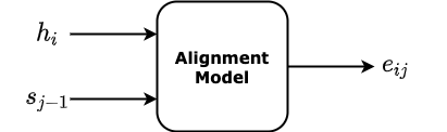
Fig.2 Block diagram showing input and output to the alignment model. \(h_i\) represents hidden state of the encoder from i-th timestep and \(s_{j-1}\) represents the hidden state of the decoder from (j-1)-th timestep. \(e_ij\) represents the alignment/compatibility between encoder and decoder hidden states.
Now the obvious question is, what is this alignment model? Well (Bahdanau et al.) decided to use a simple feed-forward neural network for this alignment model, which is further described in \eqref{eq:attention_score}. The alignment model will be called \(T_{x} \times T_{y}\) number of times to generate the alignment scores between all \(h_i\) and \(s_{j-1}\). Due to this high time complexity, the authors in (Bahdanau et al.) chose a simple model for alignment.
\[e\left(s_{j-1}, h_{i}\right)=v_{a}^{\top} \tanh \left(W_{a} s_{j-1}+U_{a} h_{i}\right) \label{eq:attention_score}\]In the above equation, alignment score e is modeled by FFNN. \(W_{a}\) and \(U_{a}\) are the weight matrices for previous decoder state \(s_{j-1}\) and input state in consideration \(h_{i}\) respectively. \(v_{a}\) is a weight vector that is learned during the training process.
Now, let’s dissect the equation \eqref{eq:attention_score} in detail. The addition of a transformed version of the decoder’s previous state \(s_{i-1}\) and input state \(h_{j}\) generates a vector. This vector is then passed through the \(tanh\) function, which squashes each value in the vector to be between -1 and +1. Each value in the vector represents the alignment in a specific dimension between the two hidden states. On the one hand, -1 represents weak alignment; on the other hand, +1 represents strong alignment. Finally, the output vector from \(tanh\) operation is element-wise element-wise multiplied with weight vector \(v_{a}\). As a final result, this element-wise multiplication is a scalar value e representing the alignment score between two hidden states. Note that this final alignment score comprises alignment between two states together in all the dimensions. Also, as a result of final element-wise multiplication, there is no restriction on the value of the final alignment score to be less than 1.
So far, we have only generated an alignment score, not a probability, i.e., it need not be between 0 and 1. Though we can get the relative importance of hidden states by directly comparing the raw alignment scores (\(e\)), if we have these alignment scores in the form of probabilities (b/w 0 and 1), it can help us determine the relative importance to place on a hidden input state. Therefore, we transform the raw scores into a probability with the help of our old-time friend \(softmax\) to squash all the generated unbounded alignment scores to be between 0 and 1.
\[\alpha_{i j}=\frac{\exp \left(e_{i j}\right)}{\sum_{k=1}^{T_{x}} \exp \left(e_{i k}\right)} \in 0 < \mathbb{R} < 1 \label{eq:alignment_weight}\]After using softmax, as an output of \eqref{eq:alignment_weight} we get \(\alpha_{i j}\) which is the alignment weight between hidden state \(h_{i}\) for the prediction of target word \(y_{j}\). Finally, our dynamic context vector should weigh each hidden state ( \(h_{i}\) ) based on this alignment weight (i.e., \(\alpha_{i j}\) ). This is accomplished by simply scaling (i.e., multiplying) n-dimensional encoded hidden representation of input word \(h_i\) with the alignment weight \(\alpha_{i j}\) as formulated below in \eqref{eq:dynamic_context_vector}.
\[c_{j}=\sum_{i=1}^{T_{x}} \alpha_{i j} h_{i} \in \mathbb{R}^{n} \label{eq:dynamic_context_vector}\]If you have followed me so far, now you should realize that in \eqref{eq:dynamic_context_vector}, we have accomplished something magical, i.e., dynamic context vector. Specifically, when we add together encoder hidden states (\(h_i\)) weighted by the alignment score (\(\alpha_{ij}\)), we get a dynamic context vector (\(c_j\)). This dynamic context vector can now guide the decoder on which part of the input sequence to focus.
To help us visualize better the series of steps involved in calculating the dynamic context vector \(c_{j}\) from all the encoder hidden states \(h_1, h_2, .. , h_{T_x}\) and decoders previous hidden state \(s_{i-1}\) refer the Fig. 3 below.
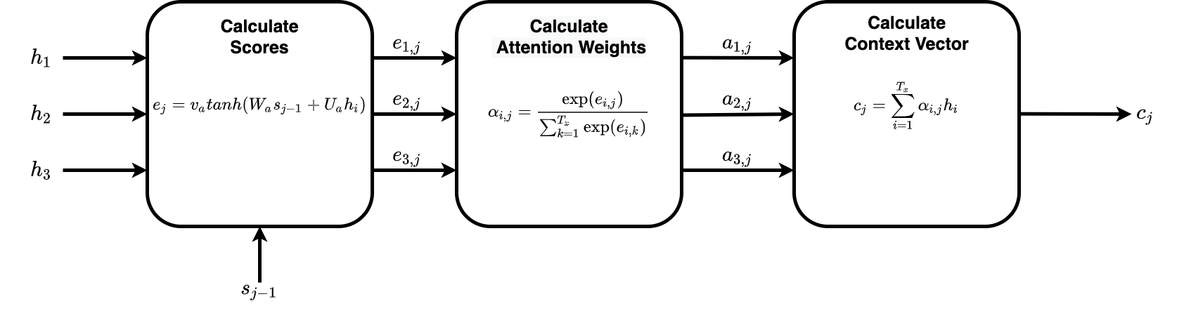
Fig. 3 details how the dynamic context vector \(c_j\) is calculated from encoder hidden state \(h_i\) and previous decoder’s hidden state \(s_{j-1}\). \(i\) and \(j\) are used as indexes for the encoder and decoder hidden states, respectively.
Now that we have seen how to calculate the dynamic context vector \(c_j\) in \eqref{eq:dynamic_context_vector}, let’s substitute its value back in \eqref{eq:attention_decoder_hidden_state} and finally in \eqref{eq:attention_decoder} to generate the distribution over the target words \(y_j\). Below, Fig. 4 helps us visualize the flow of information to first calculate decoder’s current hidden state \(s_j\), based on decoder’s previous hidden state \(s_j-1\) and dynamic context vector for the current timestep \(c_j\), which is later used along with dynamic context vector \(c_j\) and previous target word \(y_{j-1}\) to generate final distribution over target word’s probability for the current time step.
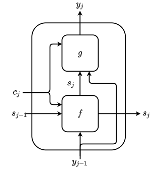
Fig. 4 Steps to first calculate the decoder’s hidden state \(s_j\) and target word probability \(y_j\)
Below, Fig. 5 shows all the components discussed so far together. It shows how the encoder and decoder hidden states help determine the dynamic context vector, which later helps determine the distribution of the words in the target vocabulary.
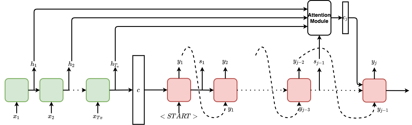
Fig. 5 Sequence to Sequence Diagram using Attention Module in the Decoder
To summarize, we first saw the conventional encoder-decoder architecture proposed for the task of NMT. Later we delved deep into the internals and working of the encoder and decoder of this architecture. We last discussed when the encoder squashes all the information from the input sequence in a single fixed-length context vector, and later decoder generating words based on that one context vector introduces a bottleneck problem. We then presented an attention mechanism that was proposed to solve the bottleneck problem. We then discussed different components of the attention mechanisms, such as the alignment model and calculating attention weights. Finally, we saw how this dynamic context vector could help resolve the bottleneck problem by conditioning the distribution of the words in the target vocabulary over the dynamic context vector.
Cited as:
@article{daultani2021attention,
  title   = "Demystifying Attention!",
  author  = "Daultani, Vijay",
  journal = "https://github.com/vijaydaultani/blog",
  year    = "2021",
  url     = "https://vijaydaultani.github.io/blog/2021/10/08/demystifying-attention.html"
}
If you notice mistakes and errors in this post, don’t hesitate to contact me at [vijay dot daultani at gmail dot com], and I would be pleased to correct them!
See you in the next post :D
References
[1] Dzmitry Bahdanau and Kyunghyun Cho and Yoshua Bengio. “Neural machine translation by jointly learning to align and translate.” ICLR 2015.
[2] Ilya Sutskever and Oriol Vinyals and Quoc V. Le “Sequence to Sequence Learning with Neural Networks” NIPS 2014.
[3] Alex Graves “Attention and Memory in Deep Learning”
[4] Lilian Weng “Attention? Attention!”